
Like most folks in the computer vision and machine learning community, I’ve recently been using deep neural networks in my research. Deep learning has attracted huge amounts of interest recently as they have managed to achieve state-of-the-art results in many sub-domians of computer vision such as classification, localisation, segmentation and action recognition to name a few. Most notably, deep learning has recently been able to surpass human level performance on the incredibbly difficult ImageNet challenge. The beautiful thing about deep learning, is that these systems learn purely from the data, so called end-to-end learning, using a simple optimization technique called gradient descent
Gradient descent is an optimization algorithm used to find a local (or the global if you’re lucky!) minimum of a function. In terms of machine learning, if we can express the goal of our algorithm with a error function (sometimes called a cost function), $E(x)$, then the global minimum of this function will give us the point of minimal error, which is exactly what we want our algorithm to achieve!
To illustrate this, lets take the traditional example of simple linear regression i.e. fitting the line of best fit to some data. Let’s assume we have the following data points $(y_i, x_i)$ as plotted below.
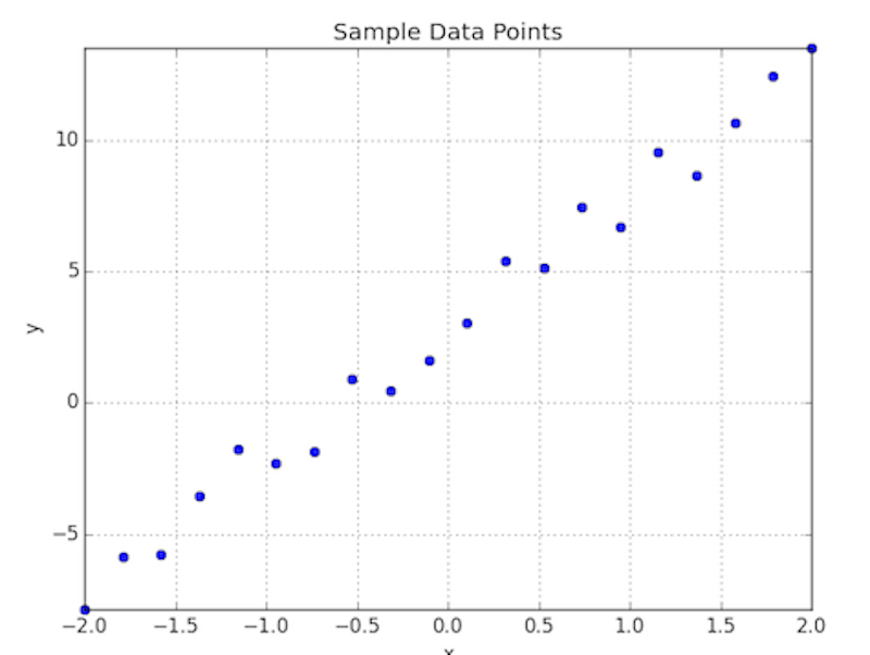
We want to fit a straight line to this data, recall that the function for a straight line is
So given the data above, we are trying to find the coefficients $m$ and $b$ that best represent our data. To measure how well an estimate of $m$ and $b$ represent our data, we must define an error function over these coefficients, $E\left(m,b\right)$. In this example, we will use the average sum of squared differences for our error function, which essentially squares the error between the predicted value ($mx_i + b$) and the actual value ($y_i$), for each of the $N$ data points, $(y_i, x_i)$, in our dataset. More formally, $E(m,b)$ is defined as:
As our error function is only defined over 2 variables, we can visualize it for our data as shown below. As we can see there’s an obvious global minimum on this surface around the point where $\left(m = 5, b = 3\right)$, which is precisely the parameters used to generate the toy data points above.
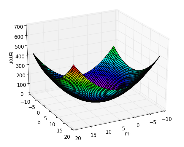
The goal of gradient descent is to start on a random point on this error surface $(m_0, b_0)$ and find the global minimum point $\left(m^{\ast}, b^{\ast}\right)$. Recall that the gradient at a point is the vector of parital derivates $\left(\frac{\partial E}{m}, \frac{\partial E}{b}\right)$, where the direction represents the greatest rate of increase of the function. Therefore, starting at a point on the surface, to move towards the minimum we should move in the negative direction of the gradient at that point. This is precisely what gradient descent does. More formally, gradient descent is an iterative algorithm described by the following steps:
- Use estimates of parameters $(m_j, b_j)$ to calculate the error $E(m_j, b_j)$
- Calculate the partial derivatives $\frac{\partial E}{m_j}$ and $\frac{\partial E}{b_j}$
- calculate the new estimates: $$ m_{j+1} = m_j - \gamma\frac{\partial E}{m_j} \\ b_{j+1} = b_j - \gamma\frac{\partial E}{b_j} \\ $$
Notice the $\gamma$ variable in Step 3 above, this is called the learning rate, which controls the effect of each movement the variables make.
So as you can see, the difficulty lays in the ability to calculate the partial derivatives of the error function, with respect to our parameters. For our example error function above we get the following results:
Now all we need to do is determine the learning rate to use (which is the topic of a field called hyperparameter optimization) and how many steps to perform gradient descent for. Below, are the results for applying gradient descent for $20$ steps with a learning rate of $0.01$ from the starting point $(m=-8, b=-8)$, as you can see we obtain a pretty good estimate of the underlying function. Ideally, we would evaluate this against a validation set to get a gauge of how well our estimate generalizes, but for these toy examples I think eyeballing the resulting function will suffice.
$20$ steps of gradient descent with learning rate of $0.01$
Let’s take another example, this time our dataset is drawn from the function $y_i = -4 + 3x +4x^2 + 4x^3$, with some jitter of $\pm 5$ applied, as shown below.
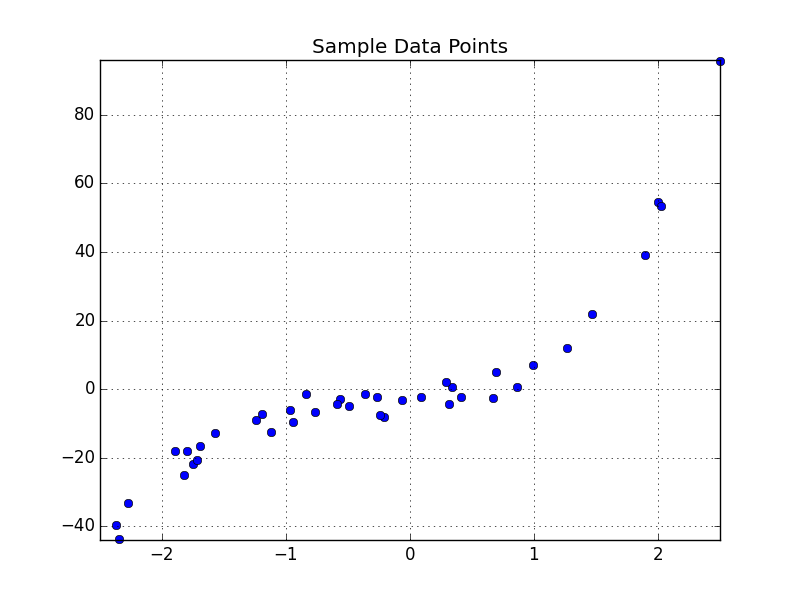
This function is a $3^{rd}$ degree polynomial, so we will try to use gradient descent to fit a function of the form shown below to the data.
Where $a…d$ are the coefficients we want to predict. Therefore, given our $N$ data points, $(y_i, x_i), our error function over these coefficients is defined as:
\[E\left(a,b,c,d\right) = \frac{1}{N} \sum_{i=1}^{N}\big(y_i - f(x_i)\big)^2\]Unfortunately, as the error is defined over 4 variables, we cannot visualize the 4-dimensional error surface. All that remains, is to define the partial derivatives $\frac{\partial E}{a}…\frac{\partial E}{d}$, which are:
\[\frac{\partial E}{a} = -\frac{2}{N}\sum_1^{N} \big(y_i - f(x_i)\big) \qquad \frac{\partial E}{b} = -\frac{2}{N}\sum_1^{N} x_i\big(y_i - f(x_i)\big) \\ \frac{\partial E}{c} = -\frac{2}{N}\sum_1^{N} x_i^2\big(y_i - f(x_i)\big) \qquad \frac{\partial E}{d} = -\frac{2}{N}\sum_1^{N} x_i^3\big(y_i - f(x_i)\big)\]Finally, below are the results of $100$ steps of gradient descent with a learning rate of $0.03$, starting from the point $(0, 0, 0, 0)$ in the error space.

While its encouraging to see that we are obtaining good results using the gradient descent technique, there is something that we have glossed over. If your error surface is convex and with an appropriate learning rate (i.e. not too high), then convergence to the global minima is guaranteed. However, in many real-world problems, the error surface is generally highly non-convex, meaning there are a plethora of local minima. In this situation, depending on the initial parameters we choose, the solution could converge to a local minima that is not neccesarilly the global minima. Whilst this non-convexity is typical of many real-world problems, don’t let that discourage you. In fact, gradient descent is still used in practice, and is the most popular technique used in training deep neural networks, they just use with a few tricks such as smart initialization of parameters and momentum to name a few.
Finally, If you want to re-produce the results from above, you can find the code used for this on my github here.